regstats
Regression diagnostics
Description
Examples
Load the patients data set, which contains simulated data on 100 hospital patients.
load patientsPerform a multiple linear regression of the Diastolic values on the Height, Weight, and Age predictors. Return all available diagnostic statistics in the structure stats.
stats = regstats(Diastolic,[Height Weight Age])
stats = struct with fields:
        source: 'regstats'
             Q: [100×4 double]
             R: [4×4 double]
          beta: [4×1 double]
          covb: [4×4 double]
          yhat: [100×1 double]
             r: [100×1 double]
           mse: 46.9215
       rsquare: 0.0533
    adjrsquare: 0.0237
      leverage: [100×1 double]
        hatmat: [100×100 double]
          s2_i: [100×1 double]
        beta_i: [4×100 double]
      standres: [100×1 double]
       studres: [100×1 double]
       dfbetas: [4×100 double]
         dffit: [100×1 double]
        dffits: [100×1 double]
      covratio: [100×1 double]
         cookd: [100×1 double]
         tstat: [1×1 struct]
         fstat: [1×1 struct]
        dwstat: [1×1 struct]
The stats structure contains diagnostic statistics for the regression fit. To access individual statistics, use dot notation. For example, stats.beta displays the regression coefficients.
stats.beta
ans = 4×1

   72.3544
   -0.0064
    0.0571
    0.0585
Load the hald data set, which measures the effect of cement composition on its hardening heat.
load haldThis data set includes the variables ingredients and heat. The matrix ingredients contains the percent composition of four chemicals present in the cement. The vector heat contains the values for the heat hardening after 180 days for each cement sample.
Fit a multiple linear regression model to the data. Use a model that includes interaction terms, and return only the fitted values and residuals to the structure stats.
stats = regstats(heat,ingredients,"interactions",["yhat" "r"])
stats = struct with fields:
    source: 'regstats'
      yhat: [13×1 double]
         r: [13×1 double]
Plot the residuals versus the fitted heat values, and add a red dashed line to indicate the mean residual value.
scatter(stats.yhat,stats.r)
ylabel("Residual")
xlabel("Fitted Heat Value")
hold on
yline(mean(stats.r),"r--")
hold off
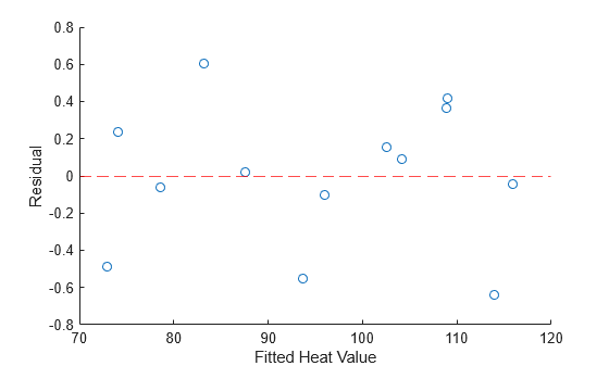
The plot shows that the mean residual value is close to 0, and that the residual values range from –0.7 to 0.6.
Input Arguments
Response variable, specified as an n-by-1 numeric vector, where
n is the number of rows (observations) in X.
Each entry in y is the response for the corresponding row of
X. The software treats NaN values as missing
values, and omits observations with missing response values from the regression
fit.
Data Types: single | double
Predictor variables, specified as an n-by-p
numeric matrix, where n is the number of observations and
p is the number of predictor variables. Each column of
X represents one variable, and each row represents one
observation.
By default, the model includes a constant term unless you explicitly remove it, so
do not include a column of 1s in X.
The software treats NaN values as missing values, and omits
observations with missing values from the regression fit.
Data Types: single | double
Model terms, specified as a value in the following table or as a numeric matrix.
| Value | Model Contents |
|---|---|
"linear" or "additive"
(default) | Constant and linear terms |
"interactions" | Constant, linear, and interaction terms |
"quadratic" | Constant, linear, interaction, and squared terms |
"purequadratic" | Constant, linear, and squared terms |
If you specify modelspec as a numeric matrix, it must contain
one column for each predictor and one row for each polynomial term in the model. The
entries in each row are exponents for the predictors in the columns of
X. For example, if a model has predictors X1,
X2, and X3, then row [0 1 2]
in modelspec specifies the term
X10X21X32.
A row of all zeros in modelspec specifies a constant term, which
can be omitted.
Data Types: single | double | char | string
Names of the diagnostic statistics to compute, specified as a character vector,
string array, or cell array of character vectors. You can specify any combination of
values in the following table, or specify "all" to compute all of the
statistics.
| Value | Description | More Information |
|---|---|---|
Q | Q from the QR decomposition of the design matrix | See Factorizations |
R | R from the QR decomposition of the design matrix | |
beta | Regression coefficients | See What Is a Linear Regression Model? |
yhat | Fitted values of the response data | |
covb | Covariance of regression coefficients | See Coefficient Standard Errors and Confidence Intervals |
mse | Mean squared error | |
r | Residuals | See Residuals |
studres | Studentized residuals | |
standres | Standardized residuals | |
rsquare | R2 statistic. This statistic might be negative for models without a constant term, which indicates that the model is not appropriate for the data. | See Coefficient of Determination (R-Squared) |
adjrsquare | Adjusted R2 statistic | |
leverage | Leverage | See Hat Matrix and Leverage |
hatmat | Hat matrix | |
s2_i | Delete-1 variance | See Delete-1 Statistics |
beta_i | Delete-1 coefficients | |
dfbetas | Scaled change in regression coefficients | |
dffit | Change in fitted values | |
dffits | Scaled change in fitted values | |
covratio | Change in covariance | |
cookd | Cook's distance | See Cook’s Distance |
tstat | t statistics and p-values for coefficients | See F-statistic and t-statistic |
fstat | F-statistic and p-value. The software computes this statistic with the assumption that the model contains a constant term. The F-statistic is incorrect for models without a constant term. | |
dwstat | Durbin-Watson statistic and p-value | See Durbin-Watson Test |
| all | All supported statistics |
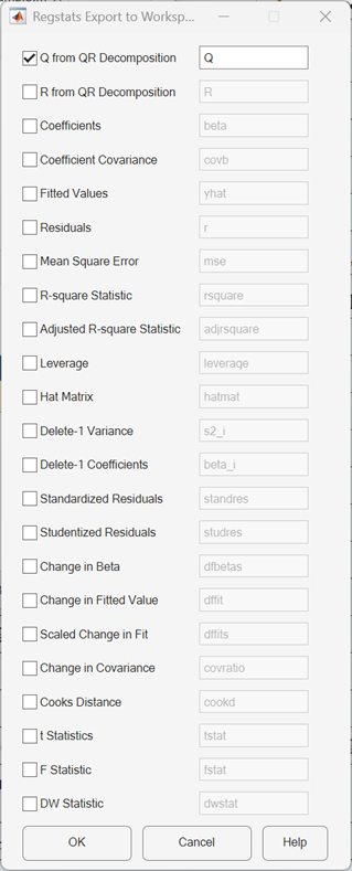
If you do not specify StatNames or return
stats, the function displays a dialog box that contains a list of
supported diagnostic statistics. The names of the workspace variables are displayed on
the right-hand side of the interface. You can change the name of a workspace variable to
any valid MATLAB® variable name. When you select check boxes corresponding to the statistics
you want to compute and click OK, the function returns the
selected statistics to the MATLAB workspace as variables.
Data Types: string | char | cell
Output Arguments
References
[1] Belsley, D. A., E. Kuh, and R. E. Welsch. Regression Diagnostics. Hoboken, NJ: John Wiley & Sons, Inc., 1980.
[2] Chatterjee, S., and A. S. Hadi. "Influential Observations, High Leverage Points, and Outliers in Linear Regression." Statistical Science. Vol. 1, 1986, pp. 379–416.
[3] Cook, R. D., and S. Weisberg. Residuals and Influence in Regression. New York: Chapman & Hall/CRC Press, 1983.
[4] Goodall, C. R. "Computation Using the QR Decomposition." Handbook in Statistics. Vol. 9, Amsterdam: Elsevier/North-Holland, 1993.
Version History
Introduced before R2006a