Reduced Order Model of a Jet Engine Turbine Blade

This example uses:

This example shows how to create a reduced order model (ROM) of a jet engine turbine blade using long short-term memory (LSTM) and neural state-space (NSS) models. You can implement the ROMs you create in Simulink® and use them for hardware-in-the-loop (HIL) testing and control design. In this example, you model the turbine blade maximum displacement when subject to variations in ambient temperature, cooling temperature, and pressure.

The high-fidelity model in this example is a MATLAB Function block. However, you can apply the example workflow to any third party finite element analysis (FEA) or computational fluid dynamics (CFD) high-fidelity model imported into Simulink as a functional mock-up unit (FMU).

In this example, you use the Reduced Order Modeler app to:

Specify ROM inputs and outputs.
Design experiments.
Generate input and output data from the Simulink model.
Train AI-based surrogate models from the input and output data using preconfigured training templates.
Implement the trained model in Simulink.

Turbine blade image.

This example requires the Reduced Order Modeler for MATLAB® add-on, which you can install using the instructions in Get and Manage Add-Ons.

For more information, see Reduced Order Modeling (Simulink).

Open Full Order Model and Reduced Order Modeler App

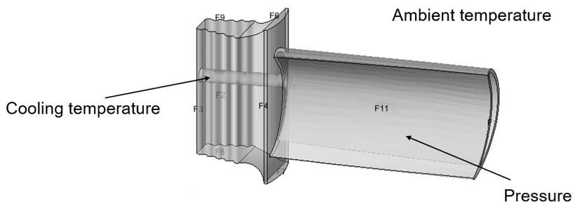
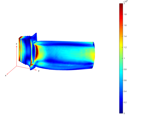
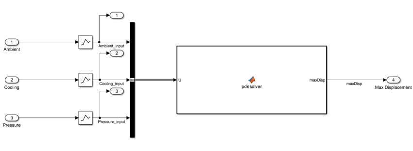
The high-fidelity model JetEngineBlade computes the displacement of a turbine blade using Partial Differential Equation Toolbox™ software through an embedded MATLAB Function block. The MATLAB Function block solves the transient heat equation to compute the temperature distribution on the blade. The block then solves a structural equation to compute the deformation or maximum displacement of the blade as a function of thermal expansion and pressure. The solve_maxDisp.m file contains the function that the block uses to compute the maximum displacement. For more information on computing maximum displacement, see Thermal Stress Analysis of Jet Engine Turbine Blade (Partial Differential Equation Toolbox).

Example Plot of the von Mises stress.

Open the Simulink model.

open_system("JetEngineBlade")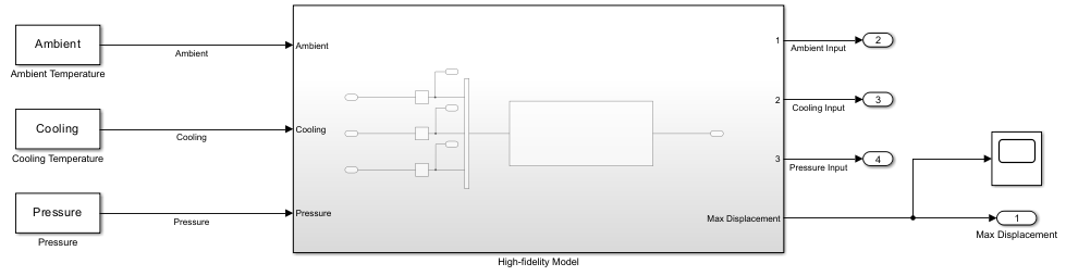

Jet Engine Blade Simulink model.

The blocks within the high-fidelity model bock in the jet engine blade simulink model.

Open the Reduced Order Modeler app.

reducedOrderModeler("JetEngineBlade")

This example describes the complete workflow to create a ROM. However, you can choose to begin at the Run Experiment step or the Create ROM Using LSTM Model step by loading the session files mentioned in these steps. These session files provide the same results as if you had completed the steps up to that point. To use reduced order models that were pretrained by following the steps in this example, begin at the Use Trained ROMs in Simulink step.

Select ROM Inputs and Outputs

Specify the ROM inputs and outputs.

In the app, on the Reduced Order Model tab, click New Session. The Select ROM I/Os dialog box opens.
In the Select ROM I/Os dialog box, click Select Signals. The Simulink model appears in a mode where you can interact with it and select signals.
To select a signal, click it in the model and then select it in the list that appears. Select the signals Ambient, Cooling, Pressure, Ambient_input, Cooling_input, Pressure_input, and maxDisp.
In the Select ROM I/Os dialog box, specify the I/O Type of the signals.

Signal	I/O Type
`Ambient`	`Simulation Input`
`Cooling`	`Simulation Input`
`Pressure`	`Simulation Input`
`Ambient_input`	`ROM Input`
`Cooling_input`	`ROM Input`
`Pressure_input`	`ROM Input`
`maxDisp`	`ROM Output`

Selecting Ambient, Cooling, and Pressure signals as simulation inputs allows you to inject random pulse sequences at these inputs and collect the ROM input and output data for each pulse sequence.

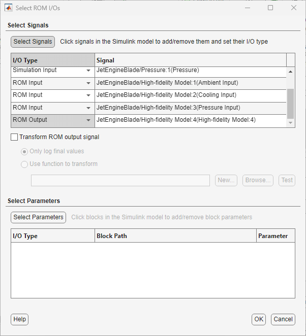
Select ROM I/Os dialog box showing the selected signals.

Click OK. The selected inputs and outputs appear in the Inputs/Outputs pane in the app.

Configure Experiment

Specify the ranges within which the simulation input signals can vary and create experiments for generating input and output data from the original model.

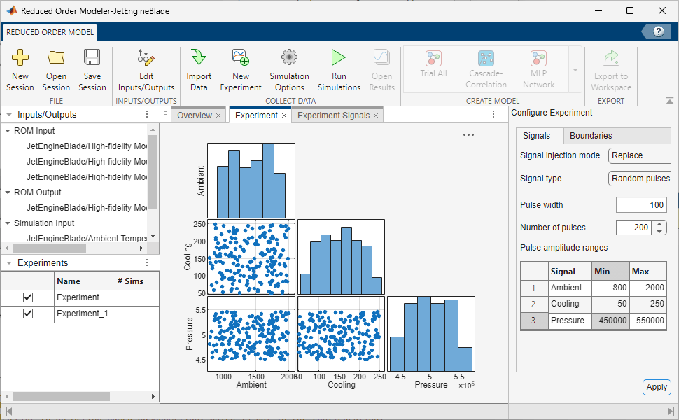
On the Reduced Order Model tab, click New Experiment. The Experiment and Experiment Signals tabs open.
To replace all simulation input signals during simulation, set the Signal injection mode to Replace in the Configure Experiment pane.
Specify Signal Type as Random pulses, Pulse width as 100, and Number of pulses as 200. Random pulses specifies that the app selects signal perturbations at random within the signal range.
Set the Min and Max values of the simulation inputs:

Signal	Min	Max
`Ambient`	`800`	`2000`
`Cooling`	`50`	`250`
`Pressure`	`450000`	`550000`

Click Apply.

To capture sufficient data to train the reduced order models, create another experiment with the same settings.

For more information on the options available to configure the experiment, see Configure Options in Reduced Order Modeler (Simulink).

Experiment tab in the Reduced Order Modeler app.

Run Experiment

Note: You can begin at this step by loading the engineBlade_ROMSession_expsetup.mat session file in the app. This session file includes the same experiment configuration as if you had completed the previous steps in the example. To load the file, on the Reduced Order Model tab, click Open Session, find the session file, and open it. To view the experiment configuration, in the Experiments pane, double-click the experiment.

Log the input and output data for training the ROM by running the engine turbine blade model with the experiments you configured.

This experiment definition produces two simulation runs, one for each experiment. If you have Parallel Computing Toolbox™ software, you can run these simulations in parallel:

On the Reduced Order Model tab, click Simulation Options.
In the Run Options dialog box, select Use Parallel when running multiple simulations.
Click OK.
If the parallel pool is not already enabled, at the MATLAB command line, type parpool('local').

To run the simulations, on the Reduced Order Model tab, click Run Simulations.

View the simulation results. To choose a simulation result to view, on the Simulation Result tab, select a simulation number in the Simulation Result box. The Result: Experiment tab shows plots of the input and output signal values from the selected simulation.

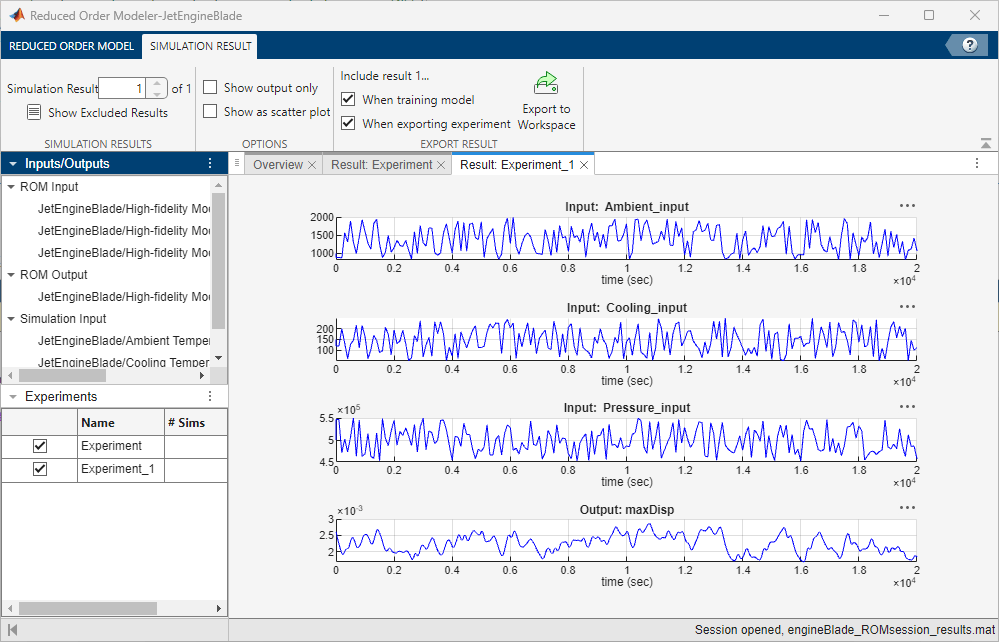
Reduced Order Modeler app showing the simulation results.

Running the high-fidelity model simulations takes a long time. You can skip to this step in the examples by opening the engineBlade_ROMsession_results.mat session file which has the pre-collected data. To view the simulation results, on the Reduced Order Model tab, click Open Results.

Create ROM Using LSTM Model

Note: You can begin at this step by loading the engineBlade_ROMSession_results.mat session file in the app. This session file contains simulation data from the jet engine blade model, collected using the same experiment configuration demonstrated in this example. To load the file, on the Reduced Order Model tab, click Open Session, find the session file, and open it. To view the simulation results, on the Reduced Order Model tab, click Open Results.

Create an LSTM model to capture the system dynamics and predict maximum displacement based on the values of ambient temperature, cooling temperature, and pressure.

First, open the Experiment Manager app:

On the Reduced Order Model tab, in the Create Model gallery, select LSTM Network as the model type.
In the Export Results dialog box, select all experiments and signals and click OK.
In the Create Experiment dialog box, select New Project, click OK, and save the experiment project. Experiment Manager opens.

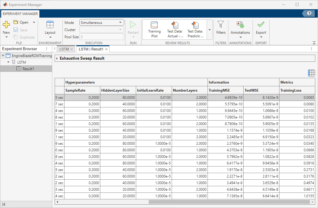
Experiment Manager creates an experiment to train LSTM models using the selected ROM input and output signals and the results of the selected experiments. In the Experiment Browser pane, right-click Experiment1 and click Rename. Rename the experiment as LSTM. To view experiment information such as the high-fidelity system, ROM model type, and test data percentage in Experiment Manager, view the Description text box on the LSTM tab.

Set the Hyperparameters Strategy to Exhaustive Sweep. Experiment Manager sweeps over different hyperparameters to train different models, then determines which models work best. Set the hyperparameters:

SampleRate — [0.2]
HiddenLayerSize — [20 40 60 80]
InitialLearnRate — [1e-2 1e-5]
NumberLayers — [1 2]

You can also edit the function used to train the LSTM models. To open the training function, in the Training Function section, click Edit. For this example, use the default training function.

If you have Parallel Computing Toolbox software, you can run multiple trials at the same time or offload your experiment as a batch job in a cluster. To train the models in parallel, on the Experiment Manager tab, in the Execution section, set Mode to Simultaneous.

To train the models, click Run. On the LSTM | Result1 tab, each row in the results table represents a trained model. The row for each model displays each of its hyperparameter values, as well as model performance information and metrics:

TrainingMSE is the mean squared error calculated on the training data set. It is the average squared difference between the output obtained by simulating the original model and the output predicted by the trained model, using the training data values. Because the training data values were used to train the model, TrainingMSE shows how well the model fits the data used to train it.
TestMSE is the mean squared error calculated on the test data set. It is the average squared difference between the output obtained by simulating the original model and the output predicted by the trained model, using the test data values. Because the test data values were not used to train the model, TestMSE shows how well the model performs on new data.
TrainingLoss is the measure of inaccuracy of the model predictions calculated on the training data set. It shows how the model progresses by learning from the training data.

Sort the trained models by TrainingLoss in ascending order by clicking the arrow on the right of the TrainingLoss column header and selecting Sort in Ascending Order in the list that appears.

The results table in Experiment Manager containing the trained LSTM models.

Of the models you trained, export the model with low TestMSE, reasonable TrainingMSE, and low TrainingLoss. To export a model as a workspace variable, first, select its row in the results table. On the Experiment Manager tab, in the Export menu, click Training Output. Name the workspace variable trainingOutput_lstm and click OK. Because the experiments that generate the training data use random pulse sequences for the input signals, model performance might vary.

For more information on hyperparameters and metrics, see Configure Options in Reduced Order Modeler (Simulink).

Create ROM Using Discrete-Time NSS Model

Create an NSS model to capture the system dynamics and predict maximum displacement based on the values of ambient temperature, cooling temperature, and pressure.

First, create a new experiment:

On the Reduced Order Model tab, in the Create Model gallery, select Neural State Space as the model type.
In the Export Results dialog box, select all experiments and signals and click OK.
In the Create Experiment dialog box, select Existing Project and choose the project that you used to train the LSTM model. Click OK.

Experiment Manager creates an experiment to train NSS models using the selected ROM input and output signals and the results of the selected experiments, then adds the new experiment to the project. Rename this experiment as Neural State-Space.

Set the NSS hyperparameters:

NumberInputLags — [0 1]
NumberOutputLags — [0 1 2]
NumberLayers — [2 3]
HiddenLayerSize — [16 32 64]
SampleRate — [0.2]
WindowSize — 50
Overlap — 0

The general form of an NSS model is

$x [k + 1] = f (x [k], u [k])$ ,

where $x [k]$ represents the states and $u [k]$ represents the inputs. This model has zero lags and the outputs are the states themselves. If a system has fewer measured outputs than states, you augment the states of the NSS model with additional lagged states. The NSS model will then take the form

$[x [k + 1]; x [k]; . . .] = f (x [k], x [k - 1], . . ., x [k - N u m b e r O u t p u t L a g s], u [k], u [k - 1], . . ., u [k - N u m b e r I n p u t L a g s])$ ,

where the first set of states in the augmented state vector are the measured outputs and the additional lagged states are the lagged outputs.

You can also edit the function used to train the NSS model. To open the training function, in the Training Function section, click Edit. This opens the training function, where you can change additional settings, such as maximum number of epochs to use during training or the network initialization options. For this example, use the default training options.

If you have Parallel Computing Toolbox software, you can train the models in parallel. On the Experiment Manager tab, in the Execution section, set Mode to Simultaneous.

To train the models, click Run. On the Neural State-Space | Result1 tab, each row in the results table represents a trained model. The row for each model displays each of its hyperparameter values, as well as model performance information and metrics:

TrainingMSE is the mean squared error calculated on the training data set. It is the average squared difference between the output obtained by simulating the original model and the output predicted by the trained model, using the training data values. Because the training data values were used to train the model, TrainingMSE shows how well the model fits the data used to train it.
TestMSE is the mean squared error calculated on the test data set. It is the average squared difference between the output obtained by simulating the original model and the output predicted by the trained model, using the test data values. Because the test data values were not used to train the model, TestMSE shows how well the model performs on new data.
TrainingLoss is the measure of inaccuracy of the model predictions calculated on the training data set. It shows how the model progresses by learning from the training data.

The results table in Experiment Manager containing the trained NSS models.

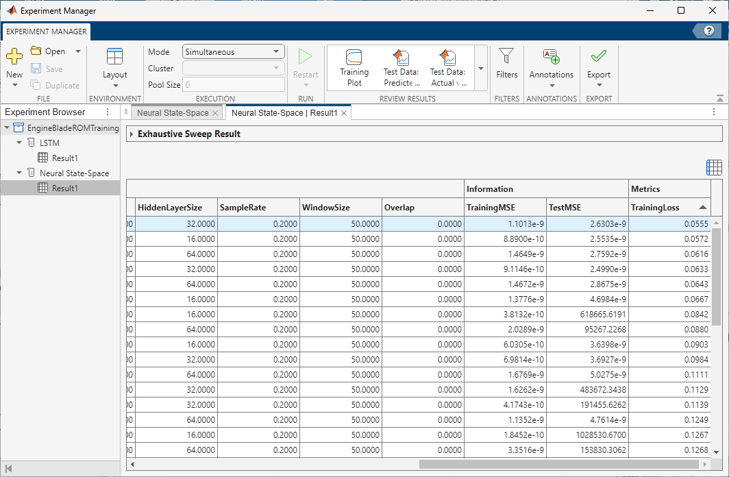
Of the models you trained, export the model with low TestMSE, reasonable TrainingMSE, and low TrainingLoss. To export a model as a workspace variable, first, select its row in the results table. On the Experiment Manager tab, in the Export menu, click Training Output. Name the workspace variable trainingOutput_nss and click OK. Because the experiments that generate the training data use random pulse sequences for the input signals, model performance might vary.

Use Trained ROMs in Simulink

Note: You can begin at this step by loading previously trained LSTM and NSS models, turbineblade_trainedLSTM.mat and turbineblade_trainedNSS.mat. These models were trained using data generated by experiments configured as shown in this example. To load the models, at the command line, enter:

load('turbineblade_trainedLSTM.mat');
load('turbineblade_trainedNSS.mat');

Warning: Updating objects saved with previous MATLAB version...
Resave your MAT files to improve loading speed.

Once you export the trained models to MATLAB workspace, you can use them in the JetEngineBlade_AI Simulink model and compare their predictions to those of the original high-fidelity model.

The trainingOutput variables store the trained models and their associated data, including normalization details.

trainingOutput_lstm

trainingOutput_lstm = struct with fields:
         TestLoss: [1×1 dlarray]
          Network: [1×1 dlnetwork]
    Normalization: [1×1 struct]

trainingOutput_nss

trainingOutput_nss = struct with fields:
         NSSModel: [1×3 idNeuralStateSpace]
      TrainingMSE: 0.0202
          TestMSE: 0.0401
    Normalization: [1×1 struct]

As part of model training, the LSTM and NSS models normalize the input and output signals. The JetEngineBlade_AI model contains blocks that normalize the input to the trained models and denormalize their output.

Model	Normalize Block	Denormalize Block
LSTM	`JetEngineBlade_AI/Normalize1`	`JetEngineBlade_AI/Denormalize1`
NSS	`JetEngineBlade_AI/Normalize`	`JetEngineBlade_AI/Denormalize`

These blocks are configured to use normalization values that are assigned to specific workspace variables. Before you open and run the model, you must extract these values from the LSTM and NSS training output and assign them to the correct variables. trainingOutput.Normalization stores the normalization data for the input and output variables.

trainingOutput_lstm.Normalization.Mu

ans=1×4 table
    Ambient_input    Cooling_input    Pressure_input     maxDisp 
    _____________    _____________    ______________    _________

       1403.7            155.3          5.0068e+05      0.0023107

trainingOutput_nss.Normalization.Mu

ans=1×4 table
    Ambient_input(t)    Cooling_input(t)    Pressure_input(t)    maxDisp(t)
    ________________    ________________    _________________    __________

         1366.7              145.55            4.9861e+05        0.0022447

Extract the input normalizations for ambient temperature, cooling temperature, and pressure and assign them to the variables specified in the normalize blocks.

meanX_lstm = trainingOutput_lstm.Normalization.Mu{1,1:3}; 
stdX_lstm = trainingOutput_lstm.Normalization.Sigma{1,1:3};
meanX_nss = trainingOutput_nss.Normalization.Mu{1,1:3}; 
stdX_nss = trainingOutput_nss.Normalization.Sigma{1,1:3};

Extract the output normalizations for maximum displacement and assign them to the variables specified in the denormalize blocks.

meanY_lstm = trainingOutput_lstm.Normalization.Mu{1,4};
stdY_lstm = trainingOutput_lstm.Normalization.Sigma{1,4};
meanY_nss = trainingOutput_nss.Normalization.Mu{1,4};
stdY_nss = trainingOutput_nss.Normalization.Sigma{1,4};

To validate the responses of the trained models, first, load turbineblade_validationData.mat. This file contains:

A set of signal values to use as input to the LSTM and NSS models.
The variable max_disp_val, which contains the prerecorded response of the high-fidelity JetEngineBlade model to these input signals.

load('turbineblade_validationData.mat')

Open the JetEngineBlade_AI model.

open_system("JetEngineBlade_AI")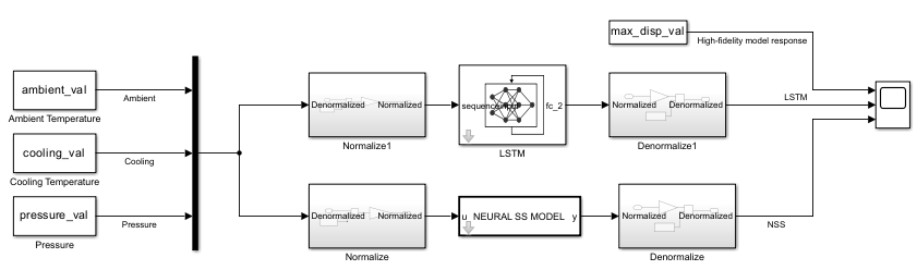

JetEngineBlade_AI simulink model

Run the model. It uses the signal values in turbineblade_validationData.mat as input. The model scope plots the maximum displacement of the blade as a function of time, as predicted by the LSTM model and the NSS model. It also uses the max_disp_val variable to plot the maximum displacement from the original high-fidelity model.

sim("JetEngineBlade_AI")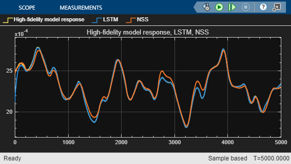

ans = 
  Simulink.SimulationOutput:

                   tout: [1001x1 double] 

     SimulationMetadata: [1x1 Simulink.SimulationMetadata] 
           ErrorMessage: [0x0 char]

The plot shows that the trained LSTM and NSS models generalize well to this data set. To further improve the model, you can:

Add additional experiments with same or different configuration settings in Reduced Order Modeler and use the data you generate to train new models.
Try different sets of hyperparameters and training options and train new models.

Once you are satisfied with the models, you can use them in Simulink for hardware-in-the-loop testing and control design, or export them for use outside of Simulink through FMUs.