T-Junction (TL)

Libraries:
Simscape /
Fluids /
Thermal Liquid /
Pipes & Fittings
Description
The T-Junction (TL) block represents a three-way pipe
junction with a branch line at port C connected at a 90° angle to
the main pipe line, between ports A and B. You
can specify a custom junction or a junction that uses a Rennels correlation or Crane
correlation loss coefficient. When Loss coefficient model is set to
Custom, you can specify the loss coefficients of each
pipe segment for converging and diverging flows.
Flow Direction
When the Loss coefficient model parameter is Crane
correlation, Rennels correlation, or
Custom, the block determines each loss coefficient
based on the flow configuration. The flow is converging when
the flow through port C merges into the main flow. The flow is
diverging when the branch flow splits from the main flow.
The flow direction between A and I, the
point where the branch meets the main, and B and
I must be consistent for all loss coefficients to be
applied. If they are not, as shown in the last two diagrams in the figure below, the
losses in the junction are approximated with the main branch loss coefficient for
converging or diverging flows.

The block uses mode charts to determine each loss coefficient for a given flow configuration. This table describes the conditions and coefficients for each operational mode.
| Flow Scenario | ṁA | ṁB | ṁC | KA | KB | KC |
|---|---|---|---|---|---|---|
| Stagnant | – | – | – | 1 or last valid value | 1 or last valid value | 1 or last valid value |
| Diverging from node A | >ṁthresh | <-ṁthresh | <-ṁthresh | 0 | Kmain,div | Kside,div |
| Diverging from node B | <-ṁthresh | >ṁthresh | <-ṁthresh | Kmain,div | 0 | Kside,div |
| Converging to node A | <-ṁthresh | >ṁthresh | >ṁthresh | 0 | Kmain,conv | Kside,conv |
| Converging to node B | >ṁthresh | <-ṁthresh | >ṁthresh | Kmain,conv | 0 | Kside,conv |
Converging to node C (branch) when the Loss
coefficient model parameter is Crane
correlation or
Custom | >ṁthresh | >ṁthresh | <-ṁthresh | (Kmain,conv + Kside,conv)/2 | (Kmain,conv + Kside,conv)/2 | 0 |
Diverging from node C (branch) when the Loss
coefficient model parameter is Crane
correlation or
Custom | <-ṁthresh | <-ṁthresh | >ṁthresh | (Kmain,div + Kside,div)/2 | (Kmain,div + Kside,div)/2 | 0 |
When the Loss coefficient model parameter Rennels
correlation, the values for converging to node C (branch) and
diverging from node C (branch) are calculated directly.
The flow is stagnant when the mass flow rate conditions do not match any defined flow scenario. Stagnant flow is permitted at the start of the simulation, but the block does not revert to stagnant flow after it has achieved another mode. The mass flow rate threshold, which is the point at which the flow in the pipe begins to reverse direction, is
where:
Rec is the Critical Reynolds number, beyond which the transitional flow regime begins.
ν is the fluid viscosity.
is the average fluid density.
Amin is the smallest cross-sectional area in the pipe junction.
Crane Correlation Coefficient Model
When you set the Loss coefficient model parameter to
Crane
					correlation
, the pipe loss coefficients,
Kmain and
Kside, and the pipe friction
factor, fT, are calculated according to
Crane [1] :
In contrast to the custom junction type, the standard junction loss coefficient is the same for both converging and diverging flows. KA, KB, and KC are then calculated in the same manner as custom junctions.
| Nominal size (mm) | 5 | 10 | 15 | 20 | 25 | 32 | 40 | 50 | 72.5 | 100 | 125 | 150 | 225 | 350 | 609.5 |
|---|---|---|---|---|---|---|---|---|---|---|---|---|---|---|---|
| Friction factor, fT | .035 | .029 | .027 | .025 | .023 | .022 | .021 | .019 | .018 | .017 | .016 | .015 | .014 | .013 | .012 |
Rennels Correlation Coefficient Model
When you set the Loss coefficient model parameter to
Rennels
					correlation
, the block calculates the pipe
loss coefficients according to [2].
The main branch diverging loss coefficient is
where:
is the mass flow rate at the inflow of the main branch.
is the mass flow rate at the outflow of the main branch.
The value of Kmain,div saturates when is equal to the value of the Minimum valid flow ratio for coefficient calculation parameter.
The side branch diverging loss coefficient is
where
is the mass flow rate at the outflow of the side branch.
d1 is the diameter of the main branch.
d3 is the diameter of the side branch.
r is the value of the Junction radius of curvature parameter.
The value of Kside,div saturates when is equal to the value of the Minimum valid flow ratio for coefficient calculation parameter.
The main branch converging loss coefficient is
where
The value of Kmain,conv saturates when is equal to the value of the Minimum valid flow ratio for coefficient calculation parameter.
The side branch converging loss coefficient is
where:
The value of Kside,conv saturates when is equal to the value of the Minimum valid flow ratio for coefficient calculation parameter.
The loss coefficient when the flow is converging to the side branch is
where d is the diameter of the side branch. The value of Kconv to side saturates when is equal to the value of the Minimum valid flow ratio for coefficient calculation parameter.
The loss coefficient when the flow is diverging from the side branch is
The value of Kdiv from side saturates when is equal to the value of the Minimum valid flow ratio for coefficient calculation parameter.
Custom T-Junction
When you set the Loss coefficient model parameter to
Custom, the block calculates the pipe loss
coefficient at each port, K, based on the user-defined loss
parameters for converging and diverging flow and mass flow rate at each port. You
must specify Kmain,conv,
Kmain,div,
Kside,conv, and
Kside,div as the Main
branch converging loss coefficient, Main branch diverging
loss coefficient, Side branch converging loss
coefficient, and Side branch diverging loss
coefficient parameters, respectively.
Constant Coefficients T-Junction
When you set the Loss coefficient model parameter to
Constant Coefficients, the block models the junction
as a composite component of three Local Resistance
(TL) blocks joined at a center node. When the block uses this
setting, it does not use mode charts. Use this option if your model operates at
nominal conditions and does not require high fidelity.
Mass and Momentum Balance
The block conserves mass in the junction such that
The block calculates the flow through the pipe junction using the momentum conservation equations between ports A, B, and C:
where I represents the fluid inertia, and
Amain is the Main branch area (A-B) parameter and Aside is the Side branch area (A-C, B-C) parameter.
Energy Balance
The block balances energy such that
where:
ϕA is the energy flow rate at port A.
ϕB is the energy flow rate at port B.
ϕC is the energy flow rate at port C.
Variables
To set the priority and initial target values for the block variables prior to simulation, use the Initial Targets section in the block dialog box or Property Inspector. For more information, see Set Priority and Initial Target for Block Variables.
Nominal values provide a way to specify the expected magnitude of a variable in a model. Using system scaling based on nominal values increases the simulation robustness. Nominal values can come from different sources, one of which is the Nominal Values section in the block dialog box or Property Inspector. For more information, see Modify Nominal Values for a Block Variable.
Examples
This example uses a test harness to compare the T-Junction (TL) and Y-Junction (TL) block behavior. A test harness is a minimally viable model that you can use to parameterize blocks or isolate dynamics.
Open Model
Open the model. The model contains both a T-Junction (TL) and Y-Junction (TL) block in two identical branches. In both blocks, identical mass flow rates enter at port B and exit from ports A and C. The dimensions of the main and side branches for both blocks are also the same.
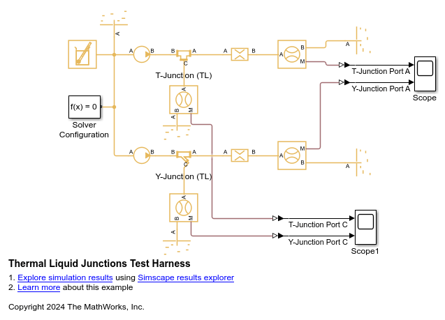
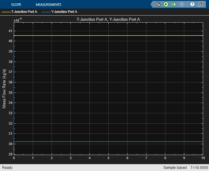
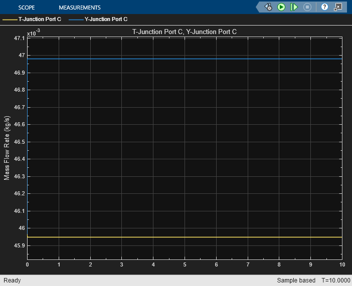
Simulation Results from Scopes
This figure shows the mass flow rate leaving from ports A and C in both blocks. The same mass flow rate that enters both blocks at port B, but in the T-Junction (TL) block, a greater portion of the flow rate exits at port A, and only a small portion exits at port C. In the Y-Junction (TL) block, a larger share of the flow that enters the block exits at port C. This is because port C leaves the main flow at an angle of 45 degrees, which is a more gradual direction change for the fluid than in the T-Junction.
Ports
Conserving
Parameters
References
[1] Crane Co. Flow of Fluids Through Valves, Fittings, and Pipe TP-410. Crane Co., 1981.
[2] Rennels, D. C., & Hudson, H. M. Pipe flow: A practical and comprehensive guide. Hoboken, N.J: John Wiley & Sons., 2012.