Autoencoders for Wireless Communications

This example shows how to model an end-to-end communications system with an autoencoder to reliably transmit information bits over a wireless channel.

Introduction

A traditional autoencoder is an unsupervised neural network that learns how to efficiently compress data, which is also called encoding. The autoencoder also learns how to reconstruct the data from the compressed representation such that the difference between the original data and the reconstructed data is minimal.

Traditional wireless communication systems are designed to provide reliable data transfer over a channel that impairs the transmitted signals. These systems have multiple components such as channel coding, modulation, equalization, synchronization, etc. Each component is optimized independently based on mathematical models that are simplified to arrive at closed form expressions. On the contrary, an autoencoder jointly optimizes the transmitter and the receiver as a whole. This joint optimization has the potential of providing a better performance than the traditional systems [1],[2].

Traditional autoencoders are usually used to compress images, in other words remove redundancies in an image and reduce its dimension. A wireless communication system on the other hand uses channel coding and modulation techniques to add redundancy to the information bits. With this added redundancy, the system can recover the information bits that are impaired by the wireless channel. So, a wireless autoencoder actually adds redundancy and tries to minimize the number of errors in the received information for a given channel while learning to apply both channel coding and modulation in an unsupervised way.

Basic Autoencoder System

The following is the block diagram of a wireless autoencoder system. The encoder (transmitter) first maps $\mathit{k}$ information bits into a message s such that $$s\in \{1,\dots ,M\}$$, where $$M=2^k$$. Then message s is mapped to n real number to create $$\text{x}=f(s)\in {\mathbb{R}}^n$$. The last layer of the encoder imposes constraints on $$\text{x}$$ to further restrict the encoded symbols. The following are possible such constraints and are implemented using the normalization layer:

• Energy constraint: $$\Vert x{\Vert }_2^2\le n$$

• Average power constraint: $$\mathbb{E}[|x_i{|}^2]\le 1,\forall i$$

Define the communication rate of this system as $$R=k/n$$ [bits/channel use], where (n,k) means that the system sends one of $$M=2^k$$ messages using n channel uses. The channel impairs encoded (i.e. transmitted) symbols to generate $$\text{y}\in {\mathbb{R}}^n$$. The decoder (i.e. receiver) produces an estimate, $$\underset{}{\overset{ˆ}{s}}$$, of the transmitted message, $$s$$.

The input message is defined as a one-hot vector $${\text{1}}_s\in {\mathbb{R}}^M$$, which is defined as a vector whose elements are all zeros except the ${\mathit{s}}^{\mathrm{th}}$ one. The channel is additive white Gaussian noise (AWGN) that adds noise to achieve a given energy per data bit to noise power density ratio, $$E_b/N_o$$.

The autoencoder maps $$k$$ data bits into $$n$$ channel uses, which results in an effective coding rate of $$R=k/n$$ data bits per channel use. Then, 2 channel uses are mapped into a symbol, which results in 2 channel uses per symbol. Map the channel uses per channel symbol value to the BitsPerSymbol parameter of the AWGN channel.

Configure Autoencoder

Choose Autoencoder

Select the autoencoder network. This example supports following autoencoder networks:

1. (2,2) Autoencoder.

2. (2,4) Autoencoder.

3. (4,4) Autoencoder.

4. (7,4) Autoencoder.

5. (8,8) Autoencoder.

selectAutoencoder = "2,2 Autoencoder";

Initialize the required parameters for autoencoder network and dataset creation

[n,k] = getAEWParameters(selectAutoencoder);
M = 2^k;  % number of possible input symbols

Train the autoencoder with an Eb/No value that is low enough to result in some errors but not too low such that the training algorithm cannot extract any useful information from the received symbols, y. Set Eb/No to 3 dB.

EbNo = 3; % Eb/No in dB
normalization = "Energy"; % Normalization "Energy" | "Average power"

Convert Eb/No to channel Eb/No values using the code rate

R = k/n;
EbNoChannel = EbNo + 10*log10(R);

As the number of possible input symbols increase, you increase the number of training symbols to give the network a chance to experience a large number of possible input combinations. The same is true for number of validation symbols.

numTrainSymbols = 2500*M;
numValidationSymbols = 100*M;

Generate Training and Validation Data

Generate random training data. Create one-hot input vectors and labels.

d = randi([0 M-1],numTrainSymbols,1);
trainSymbols = zeros(numTrainSymbols,M);
trainSymbols(sub2ind([numTrainSymbols, M], ...
  (1:numTrainSymbols)',d+1)) = 1;
trainLabels = categorical(d);

Generate random validation data. Create one-hot input vectors and labels.

d = randi([0 M-1],numValidationSymbols,1);
validationSymbols = zeros(numValidationSymbols,M);
validationSymbols(sub2ind([numValidationSymbols, M], ...
  (1:numValidationSymbols)',d+1)) = 1;
validationLabels = categorical(d);

Define Autoencoder network

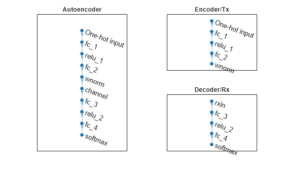
In [1], authors showed that two fully connected layers for both the encoder (transmitter) and the decoder (receiver) provides the best results with minimal complexity. Input layer (featureInputLayer) accepts a one-hot vector of length M. The encoder has two fully connected layers (fullyConnectedLayer). The first one has M inputs and M outputs and is followed by an ReLU layer (reluLayer). The second fully connected layer has M inputs and n outputs and is followed by the normalization layer (helperAEWNormalizationLayer.m). The encoder layers are followed by the AWGN channel layer (helperAEWAWGNLayer.m). The output of the channel is passed to the decoder layers. The first decoder layer is a fully connected layer that has n inputs and M outputs and is followed by an ReLU layer. The second fully connected layer has M inputs and M outputs and is followed by a softmax layer (softmaxLayer), which outputs the probability of each M symbols. The trained (n,k) wireless autoencoder network outputs the most probable transmitted symbol from 0 to M-1.

enableAnalyzeNetwork = false;

wirelessAutoEncoder = [
  featureInputLayer(M,"Name","One-hot input","Normalization","none")
  
  fullyConnectedLayer(M,"Name","fc_1")
  reluLayer("Name","relu_1")
  
  fullyConnectedLayer(n,"Name","fc_2")
  
  helperAEWNormalizationLayer("Method", normalization, "Name", "wnorm")
  
  helperAEWAWGNLayer("Name","channel", ...
    "NoiseMethod","EbNo", ...
    "EbNo",EbNoChannel, ...
    "BitsPerSymbol",2, ... % channel use per channel symbol
    "SignalPower",1)
  
  fullyConnectedLayer(M,"Name","fc_3")
  reluLayer("Name","relu_2")
  
  fullyConnectedLayer(M,"Name","fc_4")
  softmaxLayer("Name","softmax")];

wirelessAutoEncoder = dlnetwork(wirelessAutoEncoder);

Analyze the selected (n,k) autoencoder architecture.

if enableAnalyzeNetwork
    wirelessAutoEncoderAnalyzerInfo = analyzeNetwork(trainedNet);
end

Configure and Train Wireless Autoencoder

Configure Training

Configure the required hyperparameters for training the autoencoder network.

trainParams.SolverName          = "adam"; % Select the solver for training
trainParams.NumEpochs           = 10;
trainParams.MiniBatchSize       = 100*M;
trainParams.IniLearnRate        = 0.08;
trainParams.LearnRateDropPeriod = 5;
trainParams.LearnRateDropFactor = 0.1;
trainParams.LearnRateSchedule   = "piecewise";
trainParams.LossFcn             = "crossentropy";
trainParams.Metrics             = "accuracy";
trainParams.ExeEnvironment      = "cpu";
trainParams.TrainingPlot        = "none"; % Select "training-progress" to see dynamic plot of training
trainParams.EnableVerbose       = false;

options = trainingOptions(trainParams.SolverName, ...
    MaxEpochs=trainParams.NumEpochs, ...
    MiniBatchSize=trainParams.MiniBatchSize, ...
    InitialLearnRate=trainParams.IniLearnRate, ...
    LearnRateDropFactor=trainParams.LearnRateDropFactor, ...
    LearnRateDropPeriod=trainParams.LearnRateDropPeriod, ...
    LearnRateSchedule=trainParams.LearnRateSchedule, ...
    ValidationData={validationSymbols, validationLabels}, ...
    Shuffle="every-epoch", ...
    Metrics=trainParams.Metrics, ...
    ExecutionEnvironment=trainParams.ExeEnvironment, ...
    Plots=trainParams.TrainingPlot, ...
    Verbose=trainParams.EnableVerbose);

Train Autoencoder

Train the selected (n,k) autoencoder network using trainnet function.

[trainedNet, trainedNetInfo] = trainnet(trainSymbols, trainLabels, wirelessAutoEncoder, trainParams.LossFcn, options);

Split the Autoencoder

Separate the network into encoder and decoder parts.

Encoder starts with the input layer and ends after the normalization layer.

for idxNorm = 1:length(trainedNet.Layers)
    if isa(trainedNet.Layers(idxNorm), "helperAEWNormalizationLayer")
        break
    end
end
txNet = dlnetwork(trainedNet.Layers(1:idxNorm));

The decoder starts after the channel layer and ends with the softmax layer. Add a feature input layer at the beginning.

for idxChan = idxNorm:length(trainedNet.Layers)
    if isa(trainedNet.Layers(idxChan), "helperAEWAWGNLayer")
        break
    end
end
n = trainedNet.Layers(idxChan+1).InputSize;
rxNetLayers = [
    featureInputLayer(n, Name="rxin")
    trainedNet.Layers(idxChan+1:end)
    ];
rxNet = dlnetwork(rxNetLayers);

Use the plot object function of the trained network object to show the layer graphs of the full autoencoder, the encoder network, i.e. the transmitter, and the decoder network, i.e. the receiver.

figure
tiledlayout(2,2)

% Plot autoecoder network
nexttile([2 1])
plot(trainedNet)
title('Autoencoder')

% Plot encoder network
nexttile
plot(txNet)
title('Encoder/Tx')

% Plot decoder network
nexttile
plot(rxNet)
title('Decoder/Rx')  

Plot Constellation

Plot the constellation using the helperAEWPlotConstellation function. To plot the constellation of a higher order autoencoder, use t-distributed stochastic neighbor embedding (t-SNE) method. For more information, see tsne (Statistics and Machine Learning Toolbox) function.

plotTitle = string(sprintf('(%d,%d) %s', n, k, normalization));
figure
subplot(1,2,1)
helperAEWPlotConstellation(txNet)
title(plotTitle)
subplot(1,2,2)
helperAEWPlotConstellation(txNet, "t-sne")
title(plotTitle + " t-SNE")

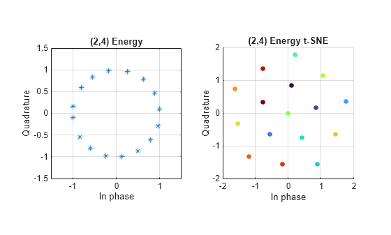
Verify the learned constellation and retrain the network if needed.

Compare Constellations

The following figure show constellations of different autoencoders.

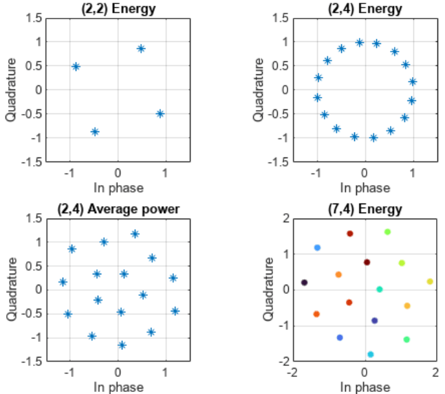
• The (2,2) autoencoder converges on a QPSK constellation with a phase shift as the optimal constellation for the channel conditions experienced.

• The (2,4) autoencoder with energy normalization converges to a 16PSK constellation with a phase shift. Energy normalization forces every symbol to have unit energy and places the symbols on the unit circle. Given this constraint, the optimal constellation is a PSK constellation with equal angular spacing between symbols.

• The (2,4) autoencoder with average power normalization converges to a three-tier constellation of 1-6-9 symbols. Average power normalization forces the symbols to have unity average power over time. This constraint results in an APSK constellation, which is different than the conventional QAM or APSK schemes. Note that, this network configuration may also converge to a two-tier constellation with 7-9 symbols based on the random initial condition used during training.

• The 2-D mapping of the 7-D constellation generated by the (7,4) autoencoder with energy constraint. 2-D mapping is obtained using the t-distributed stochastic neighbor embedding (t-SNE) method. For more information, see tsne function. (Statistics and Machine Learning Toolbox).

Simulate BLER Performance

Simulate the block error rate (BLER) performance of the selected (n,k) autoencoder. Set up simulation parameters.

simParams.EbNoVec = 0:0.5:8;
simParams.MinNumErrors = 10;
simParams.MaxNumFrames = 300;
simParams.NumSymbolsPerFrame = 10000;
simParams.SignalPower = 1;

Generate random integers in the [0 $$M$$-1] range that represents $$k$$ random information bits. Encode these information bits into complex symbols with helperAEWEncode function. The helperAEWEncode function runs the encoder part of the autoencoder then maps the real valued $$\text{x}$$ vector into a complex valued $$x_c$$ vector such that the odd and even elements are mapped into the in-phase and the quadrature component of a complex symbol, respectively, where $${\text{x}}_c=\text{x}(1:2:end)+j\text{x}(2:2:end)$$. In other words, treat the $$\text{x}$$ array as an interleaved complex array.

Pass the complex symbols through an AWGN channel. Decode the channel impaired complex symbols with the helperAEWDecode function. The following code runs the simulation for each $$E_b/N_o$$ point for at least 10 block errors. To obtain more accurate results, increase minimum number of errors to at least 100. If Parallel Computing Toolbox™ is installed and a license is available, uncomment the parfor line to run the simulations on a parallel pool.

For example, in a (2,2) configuration, the autoencoder learns a QPSK ($$M=2^k=4$$) constellation with a phase rotation as shown in the Plot constellation section.

Enable to plot the constellation learned by the autoencoder to send symbols through the AWGN channel along with the received constellation.

plotConstellation = false;

if plotConstellation
    txConst = comm.ConstellationDiagram(ShowReferenceConstellation=false, ...
        ShowLegend=true, ChannelNames={'Tx Constellation'});
    rxConst = comm.ConstellationDiagram(ShowReferenceConstellation=false, ...
        ShowLegend=true, ChannelNames={'Rx Constellation'});
end

EbNoChannelVec = simParams.EbNoVec + 10*log10(R);
BLER = zeros(size(EbNoChannelVec));

%parfor trainingEbNoIdx = 1:length(EbNoChannelVec)
for trainingEbNoIdx = 1:length(EbNoChannelVec)
  EbNo = EbNoChannelVec(trainingEbNoIdx);
  chan = comm.AWGNChannel("BitsPerSymbol", 2, ...
    "EbNo", EbNo, "SamplesPerSymbol", 1, "SignalPower", 1);

  numBlockErrors = 0;
  frameCnt = 0;
  while (numBlockErrors < simParams.MinNumErrors) ...
      && (frameCnt < simParams.MaxNumFrames)

    d = randi([0 M-1],simParams.NumSymbolsPerFrame,1);    % Random information bits
    classNames = categorical(0:M-1);
    x = helperAEWEncode(d,txNet(1));                      % Encoder
    if plotConstellation
        txConst(x)
    end
    y = chan(x);                                          % Channel
    if plotConstellation
        rxConst(y)
    end
    dHat = helperAEWDecode(y, rxNet(1), classNames);      % Decoder

    numBlockErrors = numBlockErrors + sum(d ~= dHat);
    frameCnt = frameCnt + 1;
  end
  BLER(trainingEbNoIdx) = numBlockErrors / (frameCnt*simParams.NumSymbolsPerFrame);
end

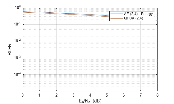
Plot the BLER results of the selected autoencoder network along with the baseline.

helperAEWPlotComparisonBLER(selectAutoencoder, n, k, normalization, BLER, simParams.EbNoVec)

Save Autoencoder

Save the trained autoencoder network and its parameters

saveToMAT = false;
if saveToMAT
    fileName = sprintf('trainedNet_n%d_k%d_%s.mat', n, k, normalization);
    saveParams.trainedNet = trainedNet;
    saveParams.txNet = txNet;
    saveParams.rxNet = rxNet;
    saveParams.info = trainedNetInfo;
    saveParams.trainParams = trainParams;
    saveParams.simParams = simParams;
    save(fileName, "-struct", "saveParams");
end

Compare BLER Performance of Autoencoders with Coded and Uncoded QPSK

The data for the following figures can be obtained using helperAEWSimulateBLER.mlx and helperAEWPrepareAutoencoders.mlx files. These show the comprison BLER performance of,

A (7,4) autoencoder and a (7,4) Hamming code with QPSK modulation for both hard decision and maximum likelihood (ML) decoding. Use uncoded (4,4) QPSK as a baseline, which is essentially a QPSK-modulated system that sends blocks of 4 bits and measures BLER.

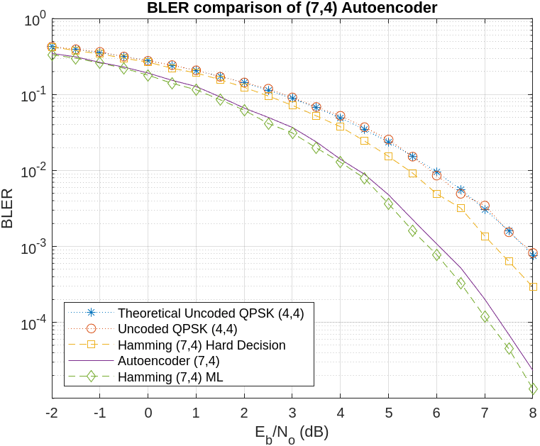
The hard decision (7,4) Hamming code with QPSK modulation provides about a 0.6 dB advantage over uncoded QPSK. While the ML decoding of the (7,4) Hamming code with QPSK modulation offers an additional 1.5 dB advantage for BLER. The BLER performance of the (7,4) autoencoder approaches that of ML decoding of the (7,4) Hamming code when trained with a 3 dB Eb/No. This BLER performance demonstrates that the autoencoder is capable of learning both modulation and channel coding, achieving a coding gain of approximately 2 dB for a coding rate of R=4/7.

Now, we compare the BLER performance of autoencoders with R=1 against uncoded QPSK systems. Use uncoded (2,2) and (8,8) QPSK as the baselines.

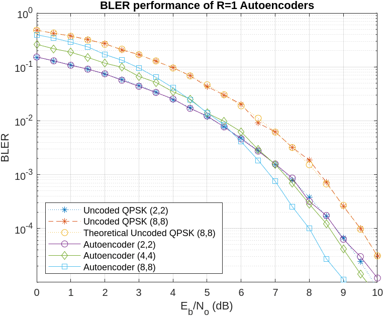
Bit error rate of QPSK is the same for both (8,8) and (2,2) cases. However, the BLER depends on the block length, $$n$$, and gets worse as $$n$$ increases as given by $$BLER=1-(1-BER{)}^n$$. As expected, BLER performance of (8,8) QPSK is worse than the (2,2) QPSK system. The BLER performance of (2,2) autoencoder matches the BLER performance of (2,2) QPSK. On the other hand, (4,4) and (8,8) autoencoders optimize the channel coder and the constellation jointly to obtain a coding gain with respect to the corresponding uncoded QPSK systems.

Effect of Training Eb/No on BLER Performance

Train the (7,4) autoencoder with energy normalization under different $$E_b/N_o$$ values and compare the BLER performance. To extend the BLER curve, set simParams.EbNoVec to 0:4.

n = 7;
k = 4;
normalization = "Energy";
traningEbNoVec = -3:5:7;
simParams.EbNoVec = 0:4;
for trainingEbNoIdx = 1:length(traningEbNoVec)
  trainingEbNo = traningEbNoVec(trainingEbNoIdx);
  [txNetVec{trainingEbNoIdx},rxNetVec{trainingEbNoIdx},infoVec{trainingEbNoIdx},trainedNetVec{trainingEbNoIdx}] = ...
    helperAEWTrainWirelessAutoencoder(n,k,normalization,trainingEbNo); %#ok<SAGROW> 
  BLERVec{trainingEbNoIdx} = helperAEWAutoencoderBLER(txNetVec{trainingEbNoIdx},rxNetVec{trainingEbNoIdx},simParams); %#ok<SAGROW> 
end

Plot the BLER performance together with theoretical upper bound for hard decision decoded Hamming (7,4) code and simulated BLER of maximum likelihood decoded (MLD) Hamming (7,4) code. The BLER performance of the (7,4) autoencoder gets closer to the Hamming (7,4) code with MLD as the training $$E_b/N_o$$ decreases from 10 dB to 1 dB, at which point it almost matches the MLD Hamming (7,4) code.

berHamming = bercoding(simParams.EbNoVec,'hamming', 'hard', n);
blerHamming = 1-(1-berHamming).^k;
hammingBLER = load('codedBLERResults');
figure
semilogy(simParams.EbNoVec,blerHamming,':k')
legendStr = sprintf('(%d,%d) Hamming HDD Upper', n, k);
hold on
linespec = {'-*','-d','-o','-s',};
for trainingEbNoIdx=length(traningEbNoVec):-1:1
  semilogy(simParams.EbNoVec, BLERVec{trainingEbNoIdx},linespec{trainingEbNoIdx})
  legendStr = [legendStr {sprintf('(%d,%d) AE - Training Eb/No=%1.1f', ...
    n, k, traningEbNoVec(trainingEbNoIdx))}]; %#ok<AGROW> 
end
semilogy(hammingBLER.simParams.EbNoVec, hammingBLER.hammingML74BLER, '--vk')
legendStr = [legendStr {'Hamming (7,4) MLD'}];
hold off
xlim([min(simParams.EbNoVec) max(simParams.EbNoVec)])
grid on
xlabel('E_b/N_o (dB)')
ylabel('BLER')
legend(legendStr{:}, 'location', 'southwest')

Conclusion and Further Exploration

The BLER results show that it is possible for autoencoders to learn joint coding and modulation schemes in an unsupervised way. It is even possible to train an autoencoder with R=1 to obtain a coding gain as compared to traditional methods. The example also shows the effect of hyperparameters such as $$E_b/N_o$$ on the BLER performance.

The results are obtained using the following default settings for training and BLER simulations:

trainParams.Plots = 'none';
trainParams.Verbose = false;
trainParams.MaxEpochs = 10;
trainParams.InitialLearnRate = 0.08;
trainParams.LearnRateSchedule = 'piecewise';
trainParams.LearnRateDropPeriod = 5;
trainParams.LearnRateDropFactor = 0.1;
trainParams.MiniBatchSize = 100*2^k;

simParams.EbNoVec = -2:0.5:8;
simParams.MinNumErrors = 100;
simParams.MaxNumFrames = 300;
simParams.NumSymbolsPerFrame = 10000;
simParams.SignalPower = 1;

Vary these parameters to train different autoencoders and test their BLER performance. Experiment with different n, k, normalization and $$E_b/N_o$$ values. See the help for helperAEWTrainWirelessAutoencoder.m, helperAEWPrepareAutoencoders.mlx and helperAEWAutoencoderBLER.m for more information.

Helper Functions

function [n,k] = getAEWParameters(autoencoderType)
%getAEWParameters Get the autoencoder parameters
%   [N,K] = getAEWParameters(autoencoderType) returns 
%   the (N,K) parameter values for selected
%   autoencoder network

% Copyright 2024 The MathWorks, Inc.

switch autoencoderType
    case "2,2 Autoencoder"
        n = 2;
        k = 2;
    case "2,4 Autoencoder"
        n = 2;
        k = 4;
    case "4,4 Autoencoder"
        n = 4;
        k = 4;
    case "7,4 Autoencoder"
        n = 7;
        k = 4;
    case "8,8 Autoencoder"
        n = 8;
        k = 8;
end
end

List of Helper Functions

• helperAEWAWGNLayer.m

• helperAEWNormalizationLayer.m

• helperAEWEncode.m

• helperAEWDecode.m

• helperAEWTrainWirelessAutoencoder.m

• helperAEWPlotConstellation.m

• helperAEWPlotTrainingPerformance.m

• helperAEWAutoencoderBLER.m

• helperAEWPlotComparisonBLER.m

• helperAEWPrepareAutoencoders.mlx

• helperAEWSimulateBLER.mlx

References

[1] T. O’Shea and J. Hoydis, "An Introduction to Deep Learning for the Physical Layer," in IEEE Transactions on Cognitive Communications and Networking, vol. 3, no. 4, pp. 563-575, Dec. 2017, doi: 10.1109/TCCN.2017.2758370.

[2] S. Dörner, S. Cammerer, J. Hoydis and S. t. Brink, "Deep Learning Based Communication Over the Air," in IEEE Journal of Selected Topics in Signal Processing, vol. 12, no. 1, pp. 132-143, Feb. 2018, doi: 10.1109/JSTSP.2017.2784180.