Tricks for Sphere Texturing
Tim
on 15 Feb 2024
Latest activity Reply by BLAISE KEVINE
on 20 Apr 2024
If you've dabbled in "procedural generation," (algorithmically generating natural features), you may have come across the problem of sphere texturing. How to seamlessly texture a sphere is not immediately obvious. Watch what happens, for example, if you try adding power law noise to an evenly sampled grid of spherical angle coordinates (i.e. a "UV sphere" in Blender-speak):
% Example: how [not] to texture a sphere:
rng(2, 'twister'); % Make what I have here repeatable for you
% Make our radial noise, mapped onto an equal spaced longitude and latitude
% grid.
N = 51;
b = linspace(-1, 1, N).^2;
r = abs(ifft2(exp(6i*rand(N))./(b'+b+1e-5))); % Power law noise
r = rescale(r, 0, 1) + 5;
[lon, lat] = meshgrid(linspace(0, 2*pi, N), linspace(-pi/2, pi/2, N));
[x2, y2, z2] = sph2cart(lon, lat, r);
r2d = @(x)x*180/pi;
% Radial surface texture
subplot(1, 3, 1);
imagesc(r, 'Xdata', r2d(lon(1,:)), 'Ydata', r2d(lat(:, 1)));
xlabel('Longitude (Deg)');
ylabel('Latitude (Deg)');
title('Texture (radial variation)');
% View from z axis
subplot(1, 3, 2);
surf(x2, y2, z2, r);
axis equal
view([0, 90]);
title('Top view');
% Side view
subplot(1, 3, 3);
surf(x2, y2, z2, r);
axis equal
view([-90, 0]);
title('Side view');
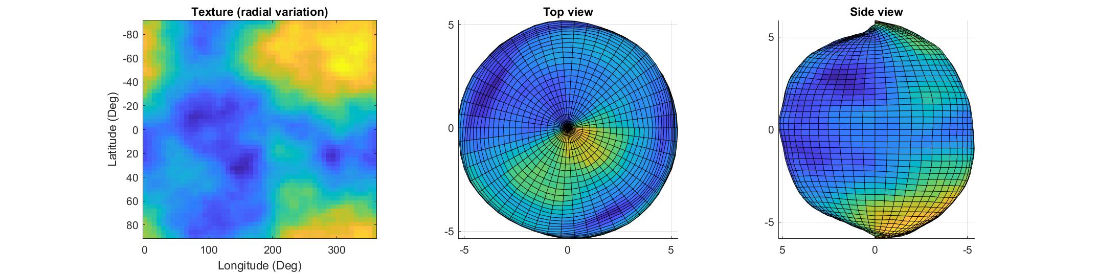
The created surface shows "pinching" at the poles due to different radial values mapping to the same location. Furthermore, the noise statistics change based on the density of the sampling on the surface.
How can this be avoided? One standard method is to create a textured volume and sample the volume at points on a sphere. Code for doing this is quite simple:
rng default % Make our noise realization repeatable
% Create our 3D power-law noise
N = 201;
b = linspace(-1, 1, N);
[x3, y3, z3] = meshgrid(b, b, b);
b3 = x3.^2 + y3.^2 + z3.^2;
r = abs(ifftn(ifftshift(exp(6i*randn(size(b3)))./(b3.^1.2 + 1e-6))));
% Modify it - make it more interesting
r = rescale(r);
r = r./(abs(r - 0.5) + .1);
% Sample on a sphere
[x, y, z] = sphere(500);
% Plot
ir = interp3(x3, y3, z3, r, x, y, z, 'linear', 0);
surf(x, y, z, ir);
shading flat
axis equal off
set(gcf, 'color', 'k');
colormap(gray);
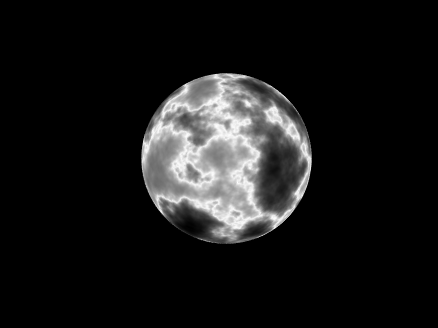
The result of evaluating this code is a seamless, textured sphere with no discontinuities at the poles or variation in the spatial statistics of the noise texture:
But what if you want to smooth it or perform some other local texture modification? Smoothing the volume and resampling is not equivalent to smoothing the surficial features shown on the map above.
A more flexible alternative is to treat the samples on the sphere surface as a set of interconnected nodes that are influenced by adjacent values. Using this approach we can start by defining the set of nodes on a sphere surface. These can be sampled almost arbitrarily, though the noise statistics will vary depending on the sampling strategy.
One noise realisation I find attractive can be had by randomly sampling a sphere. Normalizing a point in N-dimensional space by its 2-norm projects it to the surface of an N-dimensional unit sphere, so randomly sampling a sphere can be done very easily using randn() and vecnorm():
N = 5e3; % Number of nodes on our sphere
g=randn(3,N); % Random 3D points around origin
p=g./vecnorm(g); % Projected to unit sphere
The next step is to find each point's "neighbors." The first step is to find the convex hull. Since each point is on the sphere, the convex hull will include each point as a vertex in the triangulation:
k=convhull(p');
In the above, k is an N x 3 set of indices where each row represents a unique triangle formed by a triplicate of points on the sphere surface. The vertices of the full set of triangles containing a point describe the list of neighbors to that point.
What we want now is a large, sparse symmetric matrix where the indices of the columns & rows represent the indices of the points on the sphere and the nth row (and/or column) contains non-zero entries at the indices corresponding to the neighbors of the nth point.
How to do this? You could set up a tiresome nested for-loop searching for all rows (triangles) in k that contain some index n, or you could directly index via:
c=@(x)sparse(k(:,x)*[1,1,1],k,1,N,N);
t=c(1)|c(2)|c(3);
The result is the desired sparse connectivity matrix: a matrix with non-zero entries defining neighboring points.
So how do we create a textured sphere with this connectivity matrix? We will use it to form a set of equations that, when combined with the concept of "regularization," will allow us to determine the properties of the randomness on the surface. Our regularizer will penalize the difference of the radial distance of a point and the average of its neighbors. To do this we replace the main diagonal with the negative of the sum of the off-diagonal components so that the rows and columns are zero-mean. This can be done via:
w=spdiags(-sum(t,2)+1,0,double(t));
Now we invoke a bit of linear algebra. Pretend x is an N-length vector representing the radial distance of each point on our sphere with the noise realization we desire. Y will be an N-length vector of "observations" we are going to generate randomly, in this case using a uniform distribution (because it has a bias and we want a non-zero average radius, but you can play around with different distributions than uniform to get different effects):
Y=rand(N,1);
and A is going to be our "transformation" matrix mapping x to our noisy observations:
Ax = Y
In this case both x and Y are N length vectors and A is just the identity matrix:
A = speye(N);
Y, however, doesn't create the noise realization we want. So in the equation above, when solving for x we are going to introduce a regularizer which is going to penalize unwanted behavior of x by some amount. That behavior is defined by the point-neighbor radial differences represented in matrix w. Our estimate of x can then be found using one of my favorite Matlab assets, the "\" operator:
smoothness = 10; % Smoothness penalty: higher is smoother
x = (A+smoothness*w'*w)\Y; % Solving for radii
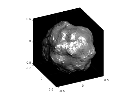
The vector x now contains the radii with the specified noise realization for the sphere which can be created simply by multiplying x by p and plotting using trisurf:
p2 = p.*x';
trisurf(k,p2(1,:),p2(2,:),p2(3,:),'FaceC', 'w', 'EdgeC', 'none','AmbientS',0,'DiffuseS',0.6,'SpecularS',1);
light;
set(gca, 'color', 'k');
axis equal
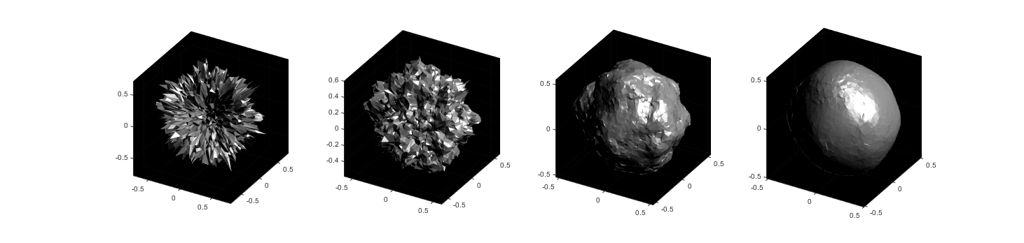
The following images show what happens as you change the smoothness parameter using values [.1, 1, 10, 100] (left to right):
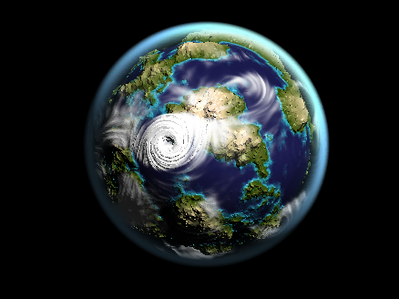
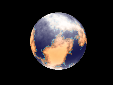
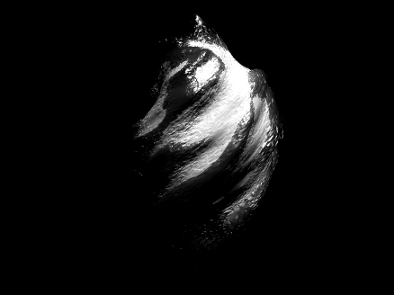
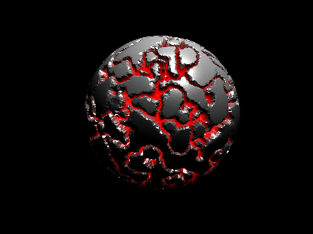
Now you know a couple ways to make a textured sphere: that's the starting point for having a lot of fun with basic procedural planet, moon, or astroid generation! Here's some examples of things you can create based on these general ideas:
5 Comments
Time Descending
Sign in to participate
SO wonderful 👍🏽👍🏽👍🏽👍🏻👍🏻
Awesome !!!
I agree with Adam and Hans. This is a great contribution!
Great article Tim!
I ran into these challenges when making my "Crates" function on the File Exchange. This makes me think that a tool to create uniform sampling on the surface of a sphere or even within a volume of a sphere would be handy.
This. Is. Awesome.